Experiment with a PID controller to control temperature

Understanding Temperature Control with PID: A Step by Step Experimentation Guide Description Meta: Learn PID temperature control using hands-on experiments. This guide provides a detailed explanation of theory, configuration, tuning (Ziegler Nichols manual), testing and analysis to help you learn process control.

1. Introduction

Precision temperature control is essential in many industries and for scientific purposes. This is crucial for maintaining product quality and enhancing efficiency in a variety of environments, from food and chemical processing, to household appliances and laboratory research. Among the most effective and widely utilised control strategies for achieving this level of accuracy and stability is Proportional-Integral-Derivative (PID) control. The PID controller's output is dynamically adjusted based on the differences between a setpoint desired (the target) and an actual process variable. This is achieved by combining three different control actions, namely Proportional Integral and Derivative. PID is a vital skill to have for any engineer or technician working in automation.

Siemens Step 7 software is a powerful and prominent programming platform that Siemens developed for their Programmable Logic Controllers. The PLCs are the core processing units of automation systems. They execute control logic, manage input/output signal and perform other functions. The step 7 environment provides an integrated platform for the development, configuration, and deployment of control strategies. This includes PID controllers. This guide is intended to provide a step-by-step, comprehensive explanation on how to implement and test a PID-based temperature control system. The entire process will be walked through, from foundational theory to hardware and software configuration, PID tuning and practical testing. This experiment aims to give a practical and clear understanding of PID Temperature Control, so that this vital but complex technology can be understood. This experiment will give learners valuable experience in PID controls, practical tuning, and how to analyze system performance.

2.Background theory: Temperature PID control

It is important to understand the fundamental principles of PID as they relate to temperature regulation before proceeding. Understanding how the PID control system's components work within a loop is crucial to its effectiveness.

A feedback control loop, at its core is an automation concept. The feedback control loop is composed of several elements that work together to keep a variable in a particular range. The loop for temperature control typically consists of a sensor that measures the current temperatures (the PV or Process Variable); a controller which contains the PID algorithm; a actuator which controls the temperature by heating or cooling; and a process which represents the actual system (e.g. a waterbath or an oven). The controller compares continuously the measured temperature PV with the desired setpoint SP. The error is the difference between the two values (E = PV - SP). This error is then used to calculate an output signal that will be sent to the actuator in order to change the temperature.

Three primary control actions are integrated into the PID controller:

Control (P) Proportional: The component produces a control result that is proportional to current error. If the temperature falls 5 degrees below setpoint then the P-action will provide a fraction of the maximum power, in proportion to the 5-degree difference. Proportional Gain Kp is used to determine the sensitivity of the response. Higher Kp values result in stronger responses to errors, which could lead to quicker adjustments. A Kp value that is too high can make the system unstable, and cause it to oscillate. A low Kp can cause a system to respond slowly and have a persistent error in the steady state, meaning that the temperature never reaches its target.

Control (I) Integral: This integral component corrects the error in steady state that is often left behind by pure proportional controls. The integral component calculates cumulative error and then adjusts output in accordance. The integral action increases (or decreases) the output control until the error has been eliminated. Integral Time Constant Ti governs the speed of the integral response. The integral time constant (Ti) is smaller, meaning that the term develops its effects more rapidly. This helps to reduce small mistakes faster. Too aggressive integral actions can lead to instability. This is especially true at the beginning of an action or when conditions change.

Control (D) Derivative: The component predicts future mistakes by analyzing the rate at which the error changes. The component measures the rate at which an error increases or decreases and takes corrective actions proportional to that rate. By counteracting changes that occur quickly in error, the derivative action can help dampen oscillations. The derivative action also helps to improve the initial response. Derivative Time Constants (Td), influence the strength of derivative actions. The predictive ability is enhanced by a larger Td, but the controller can be more sensitive to noise in the measurement. This could cause erratic changes if the tuning of the controller is not done carefully.

This equation is often used to represent the output of a PID control.

Output = Kp * E + (Ki / Td) * E dt + Kd * dE/dt

Where:

The output sends the signal to the actuator.

E (SP-PV) is an error.

Kp represents the proportional gain.

Ki represents the Integral Gain.

Kd represents the derivative gain (often expressed as Td).

E Dt is the integral error in time.

dE/dt is the change rate in the error.

In countless applications, PID controls are used to maintain temperature precisely, including heating systems, refrigerators, ovens and incubators. Tuning is the process of determining optimal values for Kp, Kd, and Ki parameters. PID controllers that are not tuned properly can have sluggish response times, overshoots, steady state errors or dangerous oscillations. Ziegler Nichols tuning involves determining the critical period and gain of the system. Manual tuning is based on the observation and adjustment of the parameters based upon the behaviour. It is important to understand these theoretical bases in order to design and implement a PID Temperature Control experiment.

Experiment Setup

For a well-planned experiment, it is important to consider the safety protocol, materials and equipment involved. This section explains the configuration and components needed to conduct the experiment on temperature control with a PID Controller.

Materials and equipment needed for an experiment depend on its complexity level and resources. A typical set-up might consist of the following.

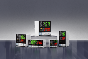
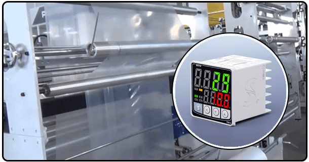
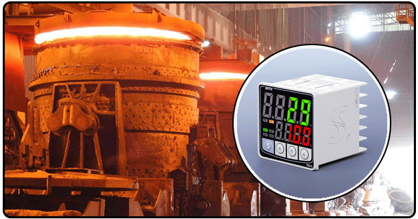
Temperature Controller The temperature controller could be a PID module or a PLC with PID built in. This controller is the brain of the system and will execute the PID algorithms.

Sensor for Temperature: The sensor measures the temperature. The most common choices are thermocouples, such as Type K or Type J, Resistance Temperature Detectors, like PT100 and PT1000 or thermistors. Selection is based on temperature ranges, accuracy and response times. Sensors must work with input channels on the controller.

Actuator An actuator is a device which physically influences the temperature of a load. Options for heating include Peltier modules that can be used to heat or cool, or solenoid vales controlling the flow of hot water. A Peltier or fan could be used for cooling. It must have the power necessary to control the temperature of the process and be controlled by the output signal from the controller.

Load Temperature: The medium or container that is controlled by the temperature. A beaker of water or a tank, a block made from metal, or a container that is empty are all examples. Load represents process to be controlled.

Power supply: Adequate power supplies must be used to power the actuator, sensor (if external power is required), and controller. They must deliver the right voltage and enough current to each component.

Data Acquisition/Measurement: Tools are needed to monitor the system's performance. Multimeters can be used to measure voltages or currents or software that is connected to controllers and sensors (e.g. via USB or Ethernet), to record data and show trends. You can use software like LabVIEW or Python, with the relevant libraries (e.g. pySerial and numpy), as well as Step 7's monitoring tools.

Software When using a PLC or microcontroller, you will need the required software development environment to compile and upload your control code. For example, Step 7 provides function blocks for PID controls (FB41 and FB42), which can be configured in the software environment.

The connections are shown in a simple block diagram. It shows the temperature sensor connected to an input channel of the controller, the actuator connected to the load (via the output channel), and finally the controller connected to the actuator. The temperature of the Load is called the Process Variable, the Setpoint is known as the Setpoint and the Controller output is Manipulated Variable which is what affects the actuator.

Any experiment that involves electrical components or temperature manipulation must be done with safety in mind. Safety precautions are:

Lockout/Tagout procedures (LOTOs) should be followed before modifying or accessing the hardware.

Wearing heat resistant gloves, safety glasses and other Personal Protective Equipment.

To prevent electric shock or short circuits, ensure that all electrical connections and cables are properly secured.

Knowing the maximum temperature that the components and load can reach safely and taking the necessary precautions (e.g. a high-temperature shutoff) if needed.

Understanding how to shut off the system safely in an emergency.

The Procedure

This procedure describes the implementation and testing step-by-step of the PID Temperature Control System. The reader is guided through the assembly of the hardware and software, the tuning of the controller, as well as the testing.

Assembly of the System: Start by connecting the components to the controller according to your chosen configuration. The temperature sensor must be physically connected to the input of the controller, the actuator should be physically attached to the output and power supplies need to go to all components. All connections must be secure and wired correctly. If you are using an Arduino board, for example, make sure that the sensor (thermistor or other) is connected to the analog input pin, and then the heating element with the appropriate transistor/mosfet and current-limiting resistance to the digital output pin.

Configuration of the software

The chosen software environment will open (e.g. Step 7, Arduino IDE or Python). New projects or workspaces can be created.

Create the project structure using step 7, and then add the symbols for temperature setpoints, sensor input, actuator out put, PID parameters, (Kp Ki Kd) and hardware configuration.

Then, add the PID function blocks (e.g. FB41 and FB42) into the program. Set its parameters such as input and output signals types, ranges, and differentiators (e.g. 0-10V for analog, 4-20mA or 0-32000 integer).

Set the input sensor channel so that the voltage or current is scaled correctly to an accurate temperature value.

Set the output channel of the actuator to the PID value calculated to match the voltage range or current range that the actuator requires.

The software will ask you to enter a value as the initial temperature setpoint. The target temperature is what you are aiming to maintain.

Initial testing: Perform initial testing after the configuration of the software and hardware to verify that the communication between the two is working.

Turn on system, ensuring that safety precautions have been observed.

Read the displayed temperature manually. If you measure it with a multimeter, does the temperature reading match that of the sensor?

Set the output manually (if you can, for example, by sending a voltage or setting a pin to high/low). The actuator should respond to your expectations.

Tuning PID Phase: In this phase, the PID (Kp) parameters are set. There are two common ways to do this:

Calculate the oscillation period and ultimate gain by using the Ziegler Nichols method. Set the Derivative Gain (Kd), and Integral Gain (Ki), to zero. Gradually increase the proportional gain (Kp), until you see the oscillation of the system with the period Pu. This is the Ku value. Ziegler Nichols can be used to estimate the initial values of Kp, Kd, and Ki (e.g. Kp = 0.6* Ku, Kp/Ti=2*Ku, Kd = 0.5* Ku/Pu, and Kp = 0.125* Ku, for example). Ziegler Nichols works best on systems of first order.

Manual tuning: Begin with the initial values of Kp, Kd and Ki. These may be based on rules-of-thumb or past experience. Change the setpoint in a small step (for example, changing the SP temperature to your new target) and watch the response of the system. Achieve a good response time without overshooting by adjusting Kp. Introduce Ki, starting with a low value to reduce steady-state errors. Finaly, add Kd to the equation (starting at a low value), in order to reduce oscillations. Many times, this process requires several iterations.

System testing: After initial tuning, perform more thorough tests in order to assess the performance of your system under various conditions.

Step-Response Test: Change the setpoint in steps (e.g. move from 25degC up to 50degC). The software can be used to record the temperatures over time. Measure and observe key performance indicators, including: the rise time, the peak overshoot, the settling time, and the steady state error.

Test for Disturbance: Create a disturbance in the system. If you are using a hot bath of water, for example, replace a large amount with cool or vice-versa. Watch how it responds. Note how fast it reaches the setpoint and if it is stable. Note down the response data. This simulation simulates a real-life scenario where process conditions can change suddenly.

Data Recording: Keep meticulous records of all the data during tuning and test phases. Included are the PID parameter values (Kp Ki Kd) chosen, setpoints, temperature measurements (steps and disturbances), as well any observations. It is recommended to use the graphing features of the software to display the controller and temperature outputs over time. This provides an excellent visual representation.

Data Analysis and Results

Outline: Recording data, plotting graphs, analysing step response (KPIs, impact of gains), analysing disturbance response, discussing tuning experience.

Content:

To evaluate the PID controller's performance and effectiveness, the collected data must be sorted and analysed. This section is devoted to interpreting results.

A. A.

Data should be presented in a systematic manner. Tables can be created to track the parameters of the PID (Kp Ki Kd), setpoints, temperature response (PV) as well as the controller output (MV). Use the trending feature of software such as Step 7 Comfort and WinCC Comfort to create graphical plots that show the temperature curve and the control signal.

B. B. Plotting the Results

Create clear graphs that clearly illustrate the performance of your system. In a typical step-response graph, temperature is plotted (y-axis), against time (x axis). For easy comparison, you can plot both the temperature response and desired setpoint on the same graph. A graph of the disturbance response will show temperature variations over time. Make sure the axes and title accurately reflect the experiment. As an example: "Step-Response Analysis: Temperature control with tuned PID controller."

C. Analyse the Step-by-Step Response

Step response analysis is used to evaluate the ability of the system to quickly and accurately reach the setpoint. The performance is quantified using Key Performance Indicators.

Rise time: Time taken for temperature to first reach setpoint. In general, a shorter rise time indicates faster reaction.

Maximum Overshoot: the maximum deviation in temperature from the setpoint. Overshoots that are excessive can cause damage to the equipment or process.

Setting Time: A time period required to maintain the temperature within the specified range of tolerance around the setpoint. The system will stabilize faster if the settling time is shorter.

Stable-State error: Difference between final temperature and setpoint, after system settles. Smaller errors indicate a better controller.

Calculate the KPIs using the graph of step-response. Discussion of the values observed and how they relate to tuning. Was the system characterized by a rapid rise time, minimal overshoot, and low steady state error? What was the impact of these PID parameters on KPIs? For example, increasing Kp could reduce the steady-state errors but increase potential overshoot. The derivative action (Kd), if it occurred, likely dampened oscillations.

D. Analyse the response to disturbances:

The robustness of the system is examined in this analysis. After the disturbance, how quickly returned the temperature to its setpoint? It is believed that a system designed well has a low deviation with rapid recovery. Discussion of the results and their relation to the tuning procedure. What was the PID controller's ability to mitigate disturbance?

E. Discussion on Tuning Experience

Consider the practical aspect of tuning a PID controller. Describe the tuning process and any difficulties encountered. Was manual tuning necessary or did the Ziegler Nichols method work well as a starting point? Iterative tuning is a good topic to discuss