Comprehensive Guide for Using PID Temperature Control

 A PID (Proportional-Integral-Derivative) temperature controller offers a powerful means to achieve precise, stable, and responsive temperature regulation. The guide explains the basics, how to use them, and their practical applications.

1. Understanding PID control: What are the fundamentals?

The PID system is fundamentally a feedback loop that automatically adjusts a process in order to keep it at a setpoint. This is done by computing an error value which represents the difference between a current measurement (process variable), and a desired value (setpoint). PID is more sophisticated than simpler methods of control. It doesn't react only to current errors, but also considers their history and forecasts future trends.

2. PID is an acronym that stands for the three components of PID.

Proportional (P). The component produces a correction proportional to the currenterror. The correction will be larger if there is a significant temperature difference. This correction's strength is determined by the 'Proportional gain', which can be denoted with Kp. Although P control is effective in implementing quick reactions, it can leave a residual error known as steady state error.

Integer (I): The Integral component is designed to eliminate the error in the steady state caused by proportional actions. The system works by adding up all the errors over time, and then applying corrections based on these accumulated errors. This accumulated error is influenced by the 'Integral Time constant' (Ti), or 'Reset Time.' Integral actions ensure that the system does not settle for long-term deviations from the setpoint.

Derived (D) This component is a look ahead. This component calculates the change rate and then applies the correction according to this calculation. A derivative action will help to slow down the process if the temperature approaches the setpoint at a rapid pace. In the opposite case, it is possible to dampen the temperature if there are rapid increases in error (indicating a potential for instability). This predictive component is controlled by the 'Derivative Time Constant (Td), or 'Derivative Gain (Kd). The derivative action is powerful, but it can also be affected by noise.

Combining these three components, a PID control can offer a nuanced, effective and efficient control strategy. This is especially true for systems that have inertia, or large delays. These are often found in temperature control.

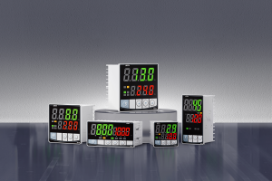
3. Building Blocks: Components in a PID System

It takes more than the PID unit to achieve precise temperature control. A complete system is required, including several essential elements.

 PID controllers are available for simple applications. Complex systems may integrate PID into a Programmable Logic Controller or Distributed Control System.

Process Sensor: Measures the temperature in the process. Thermocouples are commonly used (they have a wide range of temperature and can withstand varying temperatures) as well as Resistance Temperature Detectors. Sensors must work with controllers (e.g. input types J, K or RTD Pt100 and Pt1000).

The output device: The controller will manipulate this element to alter the temperature of the process. Examples include:

Solid State Controllers: Used to control heating elements using Pulse Width modulation (PWM) and other methods.

Setpoint: It is the target temperature the controller strives to maintain.

Feedback loop: This system uses continuous measurements (feedback), to compare actual temperatures (process variables) with the setpoint. Closed-loop control is essential for automated control.

To use a PID controller successfully, it is important to understand these components.

H2 Implementing PID control: A Step-byStep guide

Planning and execution are essential to using a PID controller. This is a guide for general implementation.

4. Define your application requirements:

What is the temperature target range? What is the accuracy required (e.g. +-0.1degC or +-1degC?

How fast can the system heat and cool?

How to Choose the Best Controller Hardware:

Choose the right temperature sensor.

Select the appropriate actuator depending on your application (heating elements power, fan sizes, valve types).

Installation:

Install the controller at a locati0n that is protected from heat or extreme conditions.

Install the power source according to manufacturer specifications and safety instructions.

Wire the thermocouple sensor with care to the input terminals of the controller, making sure that the polarity is correct and the cold junction compensation is set.

Connect the output of the controller to the actuator you have chosen, making sure the voltage/current rating is compatible. Also ensure that the wiring is safe.

Configuration:

Start the controller, and then access its settings (typically via a keyboard, buttons or an interface connected to a computer).

Choose the appropriate temperature unit (degC/degF).

Set the desired setpoint value (SP).

Set the Control Parameters:

Control Mode: Select control mode. (P, PID, PD or PI). Choose the appropriate mode for your application (often, PID will be the target or default).

Tuning parameters: Select the proportional gain (Kp), integral time (Ti), or derivative time (Td). It is usually the most complex and critical step.

Establish any limits necessary, including high/low alert points, output saturation levels (e.g. 0-100%), and safety locks if needed.

Set the desired display format, and all communication options if necessary.

Initial tuning and testing:

Simplest: Use only P control. The Proportional Gain should be adjusted until the system is able to respond quickly and without oscillations. Not the value of Kp.

Integral Action Introduced: After stable P control has been achieved, introduce Integral actions by gradually setting Ti values (or the equivalent). Integral action can help to reduce steady-state errors. Too much integral winding-up can lead to instability. As you adjust Ti, make sure that the system is stable and there are no errors.

Add a Derivative (Optional, but helpful): A derivative action improves stability and can reduce overshoot. Set a low Td and watch the response of the system. If necessary, fine-tune Ti and Td. If the derivative action is too loud or causes problems, it can be turned off.

Monitor: Pay close attention to the temperature response during tuning. You can use features such as 'Bump Testing' or small manual setpoint adjustments to evaluate performance.

H2 Tuning: Art and Science to Getting it Right

The most important step in tuning a PID is to find the right settings. Untuned controllers may cause sluggish response, oscillations or system instability. Understanding and experimenting are required to find the best Kp, Td, and Ti values. There are several methods, from trial and error to autotune features often included in modern controllers.

5. Manual tuning methods:

Step-by-Step Response Method: Change the temperature of the process or apply a disturbance known to you. Note parameters such as rise time, overshoot and settling times. The values obtained can be used to approximate tuning constants (e.g. Ziegler Nichols formulas).

Ziegler-Nichols (Test-and-Error): There are two steps. Then, increase Kp to the point where the oscillations are steady. Notate the oscillations' period (Pu). Use a table standard (such as the Ziegler Nichols tuning rule) to determine Kp, Td, and Ti. This method is effective but can also be aggressive, leading to aggressive control actions.

Cohen Coon Method: A method empirically based on data from step-response, which often produces good results when applied to processes that have significant inertia.

Automatic Tuning: Several advanced controllers have autotune features built in. They work by making a controlled, small perturbation in the system while it is running normally (e.g. a short change to the output signal). This controller analyzes and determines tuning parameters automatically based on the response. It is faster, less dangerous and requires no manual tuning.

No matter which method you choose, tuning is an ongoing process. Test the system response with conservative values. Make small adjustments and then repeat. Process noise, changes in load, system nonlinearity, and other factors can have a significant impact on performance. Periodic tuning is required.

H2 Common applications of PID temperature control

In applications that require precise temperature control, PID controllers can be found everywhere. Some common examples include:

Industrial heating: Temperature control of ovens and furnaces, kiln fusion, heat treatment processes.

Processes of Chemical Production: Temperature control in reactors, batch mixing and distillation columns.

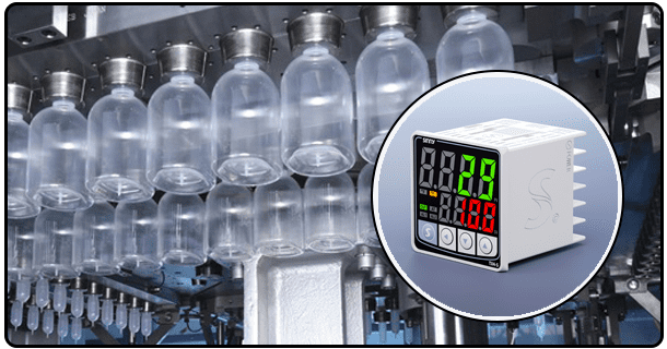
Food & Beverage: Pasteurization (ovens and proofing cabinets), sterilization, control of fermentation, freezing, freeze-drying, pasteurization.

Pharmaceutical Production: Tablet Coating, controlled Storage Environments, Lyophilization (freeze drying), Laboratory incubators.

HVAC: Climate control for clean rooms, servers rooms, data centres, laboratories and high performance buildings.

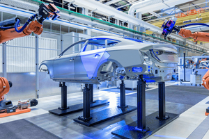
Automation and Robotics: Managing the temperature of robot joints, laser welding/cutting heads or sensitive electronic components when assembling.

Research and development: Maintaining constant temperatures for experimentation, testing of materials, and biological assays.

The ability to maintain the desired setpoint and minimize fluctuations is essential in each of these cases.

6. Troubleshooting: Maintaining Your system's performance

Problems can occur with even the best-tuned systems. These are a few common problems and their potential solutions.

Overshoot and Undershoot Persistently: System consistently overshoots or undershoots before it settles. This is often a sign of incorrect tuning. Adjust the Derivative time (Td) and Proportional gain (Kp). Increase Kp to speed the response, but reduce overshoot. Overshoot can be caused by too much integral action (Ti is not large enough).

Long Setting Time or Slow Response: It takes the system a very long time to respond to changes in setpoints or other disturbances. It could be due to an insufficient Proportional gain (Kp), or the mismatch of the controllers' capabilities with the inertia. Increase Kp may help but watch out for instability.

Oscillations Temperature swings around setpoint regularly. It is usually due to an aggressive tuning. (Too much Kp, not enough D or too little Ti) Increase the Derivative Time or Integral Time or decrease the Proportional gain (Kp).

Error of the Steady State: Temperature stabilizes to a different value than setpoint. Insufficient