


Theoretical Control of Temperature Using PID Controller Theory
I. I. Introduction to Temperature Control Systems
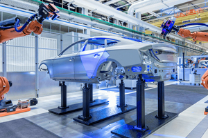
The temperature, which is a physical property of fundamental importance, has a wide range of uses, from maintaining a delicate climate in incubators to regulating commercial building's climate with massive HVAC systems. It is important to be able to control the temperature precisely. This is essential for process efficiency, product safety and compliance with regulatory requirements. For example, in industrial manufacturing it is essential to maintain optimal temperatures for chemical reactions. This will prevent unwanted byproducts and failures of the entire process. In the world of science, labs rely on stable temperatures for sensitive material experiments or exact measurements. Effective temperature control has a significant impact on comfort, indoor air quality, and energy consumption in daily contexts such as heating and cooling residential homes. Temperature control systems are designed to maintain a constant thermal setpoint in the face of changing operating conditions.
In the past, temperature regulation was done manually, which required constant monitoring and interventions. The complexity and requirements of modern processes has made automation the norm. Automated control systems provide greater precision, consistency and reliability. They can also operate without interruption, eliminating human error or fatigue. At the heart of most sophisticated automated temperature control systems lies the Proportional-Integral-Derivative (PID) controller. The powerful PID control algorithm has been developed over many decades and provides an effective framework to maintain desired conditions. It does this by continually adjusting outputs based on the differences between measured process variables and desired setpoints. It is essential to understand the theory behind PID controllers in order to design, implement, and tune effective temperature control loops. The article explores the basic principles of PID theory, and how they are applied in order to obtain accurate and stable temperatures regulation.
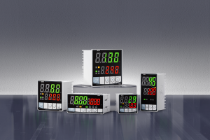
At its heart, a basic temperature control system is made up of several components that work together. The sensor is a sensor whose main function is to determine the temperature in the process. This is done by the process variable (PV),. The most common temperature sensors are thermocouples (RTDs), resistance temperature detectors, and thermistors. Each has its own range of accuracy and response speed. The controller is used to process the measurement. The controller then compares this measured PV with a target temperature that has been predefined - the Setpoint (SP).. The error is calculated by comparing the measured PV to a predefined target temperature - the strong>setpoint (SP)/strong>. This error is processed by the controller using a sophisticated algorithm based on PID. The output signal is used to control the actuator. This device can physically influence the process in order to bring the temperature closer towards the desired setpoint. The most common actuators used in temperature control are heating coils, cooling coils and fans. The final component of the temperature control system is the process itself. This could be an oven, reactor or room. This process is controlled by the actuator, while the sensor monitors the temperature. The loop closes and allows for feedback and adjustments.
Manual control is simple for simple applications, but its limits become evident in more complex and demanding situations. The human operator lacks the precision and speed required to maintain stable temperatures in dynamic environments or under tight specifications. Also, they can become tired and make mistakes. Automation, and in particular PID controllers overcome these limitations. They provide a repeatable and systematic method to achieve and maintain the desired setpoint. By calculating the corrective action based on error over time the PID controller offers a powerful way to handle the dynamics and disturbances inherent in temperature control systems. The widespread use of this controller is testament to its versatility and effectiveness.
II. The PID controller: Basic Theory
PID is the controller of choice for industrial process control because it's simple, effective, robust, and can be used in a variety of different applications. A PID controller is a simple device that calculates an output to move the process variable toward the setpoint. It does this by taking into account the current error as well as the history of previous errors and how fast the error changes. PID is the acronym for three terms that it integrates, namely Proportional Integral and Derivative.
The proportional (P), term, is by far the easiest to use. The output is proportional to current error. If the error is equal to the difference between setpoint and process variable, the mathematical formula for the proportional output is:
u_p = kp * e
Where Kp represents the proportional gains. This is a parameter which can be adjusted to determine the controller's level of sensitivity. The controller reacts more forcefully to errors with a larger Kp. The initial reaction is faster. Setting Kp to high may cause the variable to oscillate and overshoot its setpoint. The output increases when the error becomes larger, but decreases as it gets smaller. This can push the system beyond the setpoint.
The integral (I) term is used to address the problem of the steady-state errors that the proportional terms cannot completely eliminate. The error is accumulated over time, and a correction proportional to the accumulating value can be added. The integral output is calculated by:
u_i = e(tdt) * Ki
Where Ki represents the gain integral, and where the integral is equal to the sum of all the errors since the last output zero (or since startup) or the last time that the controller output has been at zero. The integral term pushes output continuously in the desired direction to remove the error. It drives the process variable toward the setpoint. The integral term adjusts the output if the error remains non-zero over any period of time. The integral term will not accumulate errors if the output of the controller reaches its limit (either maximum or minimal) due to actuator restrictions. A condition called integral woundup can occur when a high accumulated error leads to an output signal that is large and potentially damaging once the saturation level has been reached. To prevent this, careful tuning is required (often using integral time Ti or anti-windup strategy).
The derivative (D) term is focused on the future trends of the error. The derivative output (u_d) is calculated by calculating the rate of error change and adding a component that counteracts this change. The derivative output is calculated by:
u_d = Kd * de/dt
Where Kd represents the gain derived from the derivative, and where de/dt is the change rate in the error. The derivative term is used as a damping device. The derivative term can be used to prevent overshoot if the error decreases rapidly (the variable of the process is moving quickly towards the target). In the opposite case, if there is a rapid increase in error (e.g. the process variable heading rapidly away from the target), then the derivative will be added to the output to try to bring the process back to a more smooth state. The system stability is improved and the settling period (the amount of time that it takes the process variable within a band surrounding the setpoint) is reduced. The derivative term, however, is sensitive to the noise in sensor measurements. The derivative output can fluctuate dramatically if the sensor reading changes rapidly. This could lead to instability and chattering. Most modern PID controllers have a derivate filter to mitigate this. This filter reduces noise in the derivative input, resulting in a stable derivative.
This is what the output total of a PID standard controller looks like:
Output = u = u_p + u_i + u_d = Kp*e + Ki*e(t)dt + Kd*de/dt
The calculated output is then used to initiate the control of the actuator. This action will reduce any errors and return the process variable to the setpoint. Tuning, which involves adjusting Kp, Kd, or their equivalents such as Ti and Td, is critical to achieve the balance desired between the response speed, accuracy, and stability in the temperature loop.
III. Application of PID Theory for Temperature Control Loops
The feedback loop of a temperature control system is effective. Standard structure is composed of key elements that interact dynamically. Process Variable (PV). represents the current temperature within the controlled system (e.g. the temperature in an oven, a reactor). Setpoint (SP) represents the temperature desired by the controller. Sensor transmits the information to the controller. Controller compares the SP and PV to determine the error. The controller creates an output signal based on the error calculated using the PID algorithms. The actuator is controlled by this output signal. This is the last control element. For temperature, it is usually a heating or cooling element, such as a Peltier or chiller device, that reduces the temperature or a temperature valve that controls a warm or cold fluid. Actuator action influences PV directly. The closed loop of Sensor->Controller->Actuator->Process Variable->Sensor->Controller allows continuous monitoring and adjustments, which allows the system to maintain its desired temperature regardless of external disturbances such as changes in ambient temperatures or internal variations. This closed loop's effectiveness is heavily dependent on how well the PID controller implements the previously discussed theory.
Each component of PID plays an important role when it comes to maintaining SP. The proportional (P), term is the main corrective measure. The P-term is triggered when the temperature measured (PV), deviates significantly from the setpoint. The controller will add a significant amount of P to its output if the error is large. This tells the actuator to increase the power or rate. Initially correcting the error helps reduce it quickly. If the P-term alone does not eliminate the error, the integral (I) term is used. The I term gradually increases the output signal as the time goes by. This constant push will help to bring the PV ever closer to the SP and eliminate any offset. As mentioned above, it is important to manage the I term carefully in order to prevent integral windup. This becomes especially true when the actuator has reached its limits. derivative (D) term is a sophisticated addition. The D term monitors the rate at which error changes. The D term dampens the response if the error rapidly decreases (PV is quickly approaching SP). This helps to avoid overshoot. The D term will add a correction to the trend if the error increases rapidly. The system will settle faster and more easily, reducing the amount of time required to reach its setpoint. P, I and D work together to allow the PID control system to respond effectively and efficiently. This balance allows it minimize overshoot and settling times, as well as steady state error.
However, temperature systems aren't always linear. In real-life temperature processes, nonlinearity is common. The relationship between actuator inputs (e.g. heater power) can vary greatly at different operating conditions. A small setpoint change can cause large changes in temperature at low temperatures, but smaller ones at higher temperatures. It is important to apply the PID algorithm carefully, which has a linear basis, to nonlinear systems. This may require specific tuning techniques or models-based approaches. Dead Time can also be found in many temperature loops. The PV responds to a command after a certain delay. The delay can affect tuning and stability (like Ziegler Nichols). The first step to effective tuning is acknowledging these complexities. The core PID algorithm is unchanged, but the tuning must take into account these delays and non-linearities. Although the underlying PID theories provide a foundation for tuning, it is often necessary to use advanced or empirical techniques in order to account for all of these factors.
IV. The PID Control Theory of Temperature Systems: Key Concepts
Understanding key dynamics of the process and issues that may arise is essential to applying PID theory in temperature loops. The concepts can be used to select the appropriate parameters for tuning and anticipate challenges.
The Process Gain (Kp) is a measure of how sensitive a process variable to changes to the output controller. The temperature will change significantly when the actuator is adjusted. The (T) identifies the speed at which a process reacts to changes. Large time constants indicate a slower system response. The initial gains of the PID are influenced by these parameters. Dead Time (L) refers to the delay in time between an actuator's change and PV measurement. If this delay is not taken into account, it can cause the loop to become unstable. The saturation is when an actuator reaches its limits. (e.g. heaters that turn on and off without any fine control.) It can lead to integral windup whereby the I-term builds up an excessive error signal leading to extreme limits for actuators. Noise are unwanted fluctuations of the sensor signal. Thermocouples are a common example. Derivative filtering can be essential because the D term is susceptible to noise amplification. It is important to understand how these factors work with the PID algorithms for successful tuning.
V. Analysing the stability and performance of PID temperature control
Tuning a PID-loop isn't just about stabilizing the system. It also involves achieving specific performance goals. The closed-loop's ability to keep the setpoint constant without oscillating, or diverging is called stability. The ratio gain (Kp ) determines stability and response time. Kp increases response speed but can also increase instability. The integral gain (Ki), influences stability in a indirect way (through the windup of the integral) and affects steady-state performances. The derivative gain (Kd), is primarily responsible for damping and stability. Performance can be evaluated by using certain metrics.
Setting Time: the time required for the PV's to remain within a band specified around the setpoint.
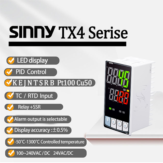
- Pid digital 12V DC temperature controller
- Digital PID temperature controller: High precision control